How we modeled Kubernetes, AWS, monitoring hosts, and time itself as a connected graph and all the work along the way.

Why We're Building a Knowledge Graph

We're building Annie, an AI-SRE that can do what a senior on-call engineer does during an incident. When an alert fires, Annie automatically correlates infrastructure changes, monitoring data, code deployments, and dependency topology to pinpoint the root cause and suggest a fix.

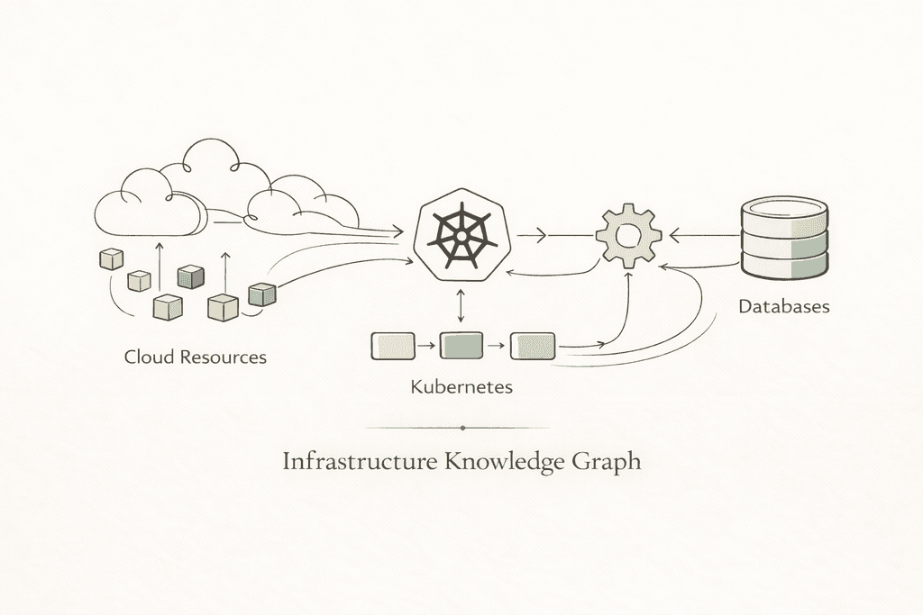
To do this, Annie needs something that doesn't exist in any single tool: a unified model of your entire prod: cloud resources, Kubernetes workloads, Terraform definitions, code changes, and monitoring signals: all connected, all versioned, all queryable across time.

That's what we call the "infrastructure knowledge graph" and building it required Neo4j.

The whole project traces back to one question: "What changed before this thing broke?" That question forces you to traverse relationships across Kubernetes, AWS, Terraform, and time simultaneously. Traditional databases can't do this at the scale and query complexity we need.

Chapter 1: The First Node

Our graph started with one node, which was the representation of an S3 bucket.

The original idea was straightforward: extract AWS resources, store them somewhere queryable and let an AI agent search through them. We picked Neo4j because infrastructure is a graph: an EC2 instance runs in a VPC, has a security group, assumes an IAM role, hosts a Kubernetes node. These aren't rows in a table but relationships in a graph.

The first version was simple: A go service pulled resources from AWS APIs, flattened their properties, and wrote them as nodes. Each node was a struct with a set of labels, a map of properties, an identifier and labels.

An S3 bucket became a node labeled something like S3_BUCKET:RESOURCE:CLOUD. An EC2 instance got EC2_INSTANCE:RESOURCE:CLOUD. Simple.

The first challenge: atomicity. The same S3 bucket exists in three places: the Terraform code that defines it, the Terraform state that tracks it, and the AWS API that runs it. Same bucket, three representations. Three different ID schemes. We needed a way to reconcile them.

This led to what we call universes: separate layers for Terraform definitions, Terraform state, live cloud APIs, Kubernetes, and so on. Each universe has its own extraction pipeline, its own identity scheme, and its own update cadence. A single resource can exist as multiple nodes across universes, linked by shared identifiers.

That cross-universe linking is where graph databases earn their keep. In a relational database, you'd need a mapping table, a reconciliation job, and a prayer. In Neo4j, it's just a relationship.

Chapter 2: Adding Kubernetes (Where Things Got Complicated)

AWS resources change slowly. You create a VPC, it sits there forever. Kubernetes is a different beast entirely.

Pods come and go, deployments roll and services shift their selectors. Across our customers, we've seen everything from small clusters with a few dozen resources that rarely change, to large production environments with thousands of resources churning every hour. When we added Kubernetes ingestion, the node count exploded: Pods, Services, ConfigMaps, Secrets, Nodes, Namespaces, Containers, ReplicaSets and every one of them needed to be connected.

The relationship types multiplied fast:

• EXPOSES: a Service exposes Pods (matched by label selectors)

• ROUTES_TO: an Ingress routes to Services

• HAS_CONTAINER: a Pod has Containers

• RUNS_ON: a K8S Node runs on an EC2 instance

• PROTECTS: a PodDisruptionBudget protects Pods

• PART_OF: everything belongs to a cluster

Challenge #2: Label selector matching. Kubernetes Services don't reference Pods by name. They use label selectors: "give me all pods where app=frontend AND tier=web." Translating this to Cypher(Neo4J query language) meant dynamically matching property keys. The idea is straightforward: find all Services in the current state, extract their selector keys, then find Pods in the same namespace whose labels satisfy every selector condition. Something like:

// Simplified example
MATCH (svc:SERVICE)
WITH svc, [k IN keys(svc) WHERE k STARTS WITH 'selector.'] AS selKeys
WHERE size(selKeys) > 0

MATCH (pod:POD {namespace: svc.namespace})
WHERE ALL(k IN selKeys WHERE pod[k] = svc[k])

MERGE (svc)-[:EXPOSES]->(pod)

This works conceptually. But it taught us something important: in a graph that models infrastructure, relationships aren't static definitions. They're computed from property matching, label selectors, ARN parsing, and naming conventions. The linking logic became its own subsystem, multiple Cypher queries handling K8s-to-K8s, K8s-to-Cloud, Terraform-to-State, State-to-Cloud, and more.

Chapter 3: The Time Problem

Here's where the story gets interesting. Knowing the current state of your infrastructure is useful. Knowing what it looked like five minutes ago right before the incident is essential. "What changed?" is the first question in every incident response. But modeling time in a graph database is a genuinely hard problem.

The naive approach: overwrite nodes on each update. Current state only. This is what we did initially, and it was useless for incident investigation. "Something changed" isn't helpful if you can't see the before and after.

The second attempt: versioned nodes. Each update creates a new node, linked to a TIME node representing when the snapshot was taken. We built a time chain:

EPOCH --NEXT--> T1 --NEXT--> T2 --NEXT--> ... --NEXT--> LAST_TIME

Every resource version connects to its corresponding time node via an [:AT] relationship. When an S3 bucket's configuration changes, a new S3 Bucket v2 node gets created, linked to the new time node. The old version stays, linked to its time. You can now query: "Show me the state of everything at T1."

This is where Neo4j's power becomes obvious. A point-in-time query that would require complex temporal joins in PostgreSQL becomes a single pattern match:

MATCH (n)-[:AT]->(t:TIME {timestamp: "2026-02-13T18:30:00Z"})
RETURN n

But the time model nearly killed our performance. Every resource, at every snapshot interval, creates a new node. At 5-minute intervals, a cluster with 200 resources generates 200 new nodes every 5 minutes. That's 57,600 nodes per day for one small cluster. For production environments with thousands of resources, we were looking at millions of nodes per month.

Challenge #3: Optimizing for "current state" queries. In practice, most queries don't ask about a specific point in time: they ask "what does everything look like right now?" Walking the full time chain to find the latest snapshot was too slow for that. We introduced a dedicated anchor node that all current-version resources point to, turning current-state lookups from a chain traversal into a direct hop.

Getting there required a migration: repointing every live node to the new anchor in batches to avoid locking the database. Small change in concept, painful change in practice.

Chapter 4: The Delta Pipeline

For months, we used snapshot-based ingestion: every sync cycle, fetch the entire cluster state, diff it against the graph, replace everything. It worked for small environments. It did not scale.

The problem: a full snapshot of a large Kubernetes cluster means processing every pod, every service, every ConfigMap; even if only one pod restarted. And during the replacement window, relationships could break. If a Service node gets deleted and recreated, the EXPOSES edge to its Pods disappears and needs to be re-linked. For a few milliseconds, your graph shows a Service with no Pods.

Challenge #4: Edge inheritance during delta updates. We built a delta pipeline that processes only changed resources and intelligently preserves relationships. The core question: when a node gets updated (effectively deleted and reinserted with new properties), what happens to its edges?

The principle is simple: carry over existing relationships to the new version of a node, unless the target is also being deleted or the relationship is being explicitly recreated by the update itself. In pseudocode:

This means when a Pod gets updated during a rolling deployment, its EXPOSES relationship from the Service survives the transition.

Getting this right was one of the hardest parts. The edge cases (pun intended) are brutal: What if both the source and target are being updated simultaneously? What if an edge was supposed to be removed by the update? What if the delta arrives out of order? We spent weeks stabilizing this, ultimately building a decision matrix that covers every combination of source state, target state, and whether the edge is already being explicitly handled.

The performance gains were massive. For a cluster where one pod restarts, that's the difference between processing hundreds of resources and processing one.

Chapter 5: The Intemporal Problem

Not everything in infrastructure changes. An AWS account doesn't have a version. A cloud region doesn't have snapshots. A Kubernetes cluster object is a permanent anchor, not a temporal resource.

But our temporal model treated everything uniformly: every node had to connect to a time node. Infrastructure "hub" nodes (accounts, regions, cloud providers, clusters) were getting swept up in retention cleanup jobs that pruned old time nodes. One morning we woke up to find cluster nodes had vanished from the graph. Not because anyone deleted a cluster because the cleanup job didn't know they were special.

Challenge #5: Hub node survival. We needed a way to mark certain nodes as exempt from the temporal lifecycle. The solution was a flag on hub nodes: accounts, regions, clusters, cloud providers that tells the cleanup process to skip them. A one-line migration:

MATCH (n)
WHERE n:CLOUD_PROVIDER OR n:ACCOUNT OR n:REGION OR n:CLUSTER
SET n.permanent = true

Flagged nodes skip the cleanup process entirely. They exist outside the time chain: permanent structural anchors that temporal resources orbit around. It's a small migration, but it solved an entire class of "where did my cluster node go?" bugs.

Chapter 6: Cross-Layer Correlation (The Real Payoff)

With Kubernetes, AWS, Terraform, and time all living in the same graph, we could finally answer the questions that motivated the entire project.

"What changed before this incident?"

A temporal traversal across deployments in a time window:

// Find deployments that changed in a time window
MATCH (d:DEPLOYMENT)-->(t:TIME)
WHERE t.timestamp >= $windowStart AND t.timestamp <= $windowEnd

// Follow the version chain to see what changed
MATCH (d)-->(d_new:DEPLOYMENT)
WHERE d.image <> d_new.image

RETURN d.name, d.image, d_new.image, t.timestamp

"Is it safe to delete this IAM user?"

A multi-hop dependency traversal: start from the user, walk through policies, groups, and compute instances to see the full impact:

MATCH (u:IAM_USER {username: 'some-user'})
OPTIONAL MATCH path = (u)-[*1..3]->(related)
RETURN u.name, [n IN nodes(path) | labels(n)] AS dependency_chain

In a relational database, this query would require joining across multiple tables with self-referential lookups and temporal filtering. In Neo4j, it's pattern matching.

"What's the blast radius of this IAM change?"

A variable-length path query: start from the IAM change, traverse through EC2 instances, to Kubernetes nodes, to Pods, to Services, to the SLA impact:

IAM Change --> EC2 (assumed_by) --> K8S Node (runs) --> Pod (hosts)
          --> Service (serves) --> API --> SLA (breaches)

This query would represent six hops, three infrastructure layers but only one query (!)

Chapter 7: Teaching an AI to Speak Cypher

The graph is only as useful as your ability to query it. We didn't want SREs writing Cypher at 3am. We wanted them to ask Annie: "What changed in the last 5 minutes that could have caused the API latency spike?"

This means an LLM needs to translate natural language into Cypher. The challenge: the LLM doesn't know your schema.

We built a schema discovery mechanism. Before generating any Cypher, the AI agent samples existing nodes for a given label and retrieves their property keys. The approach: query a sample of nodes (filtered to current state only), return the set of property keys. The LLM then sees something like: "POD has properties: name, namespace, status, nodeName, image..." and generates Cypher accordingly. Schema discovery runs on every query because the graph schema evolves as we add new resource types.

The agent architecture uses multiple specialized subagents that run concurrently during an investigation: one focuses on the infrastructure graph, another on code and deployment history, another on monitoring and alerting data. An orchestrator synthesizes findings into a root cause analysis. The graph-focused agent typically fires multiple Cypher queries per investigation, progressively narrowing from broad topology searches to precise temporal diffs.

Challenge #6: Cypher injection. When you let an LLM generate Cypher from user input, you're one prompt injection away from DETACH DELETE on your entire graph. Standard mitigations apply: input validation, query sandboxing, timeouts, and read-only transaction modes. If you're building text-to-Cypher, plan for this from day one.

What We'd Do Differently

Start with the time model. We bolted temporal support onto a static graph, and the migration pain was real. If we were starting over, the time chain would be day-one architecture.

Invest in delta pipelines earlier. Snapshot-based ingestion is fine for prototyping. It doesn't survive contact with a production Kubernetes cluster that churns 50 pods per hour.

Design for the query, not the data. The graph schema should be shaped by the questions you need to answer, not by the structure of the source APIs. We restructured our node properties three times before landing on a model that Cypher could query efficiently.

Don't underestimate the linking problem. Extracting resources is the easy part. Connecting them: across infrastructure layers, across universes, across time is where the real engineering lives. The code that creates and maintains relationships is more complex than all the extraction pipelines combined.

Why Neo4j

People ask why we chose Neo4j over PostgreSQL with recursive CTEs, or MongoDB with $graphLookup, or even a custom solution.

The honest answer: Cypher expressiveness. A 6-hop traversal spanning Kubernetes topology, AWS IAM chains, temporal versions, and Terraform state with filtering at each hop is 10 lines of Cypher. The equivalent SQL would be 100+ lines of recursive CTEs and temporal joins that no one would maintain.

The LAST node optimization, variable-length path queries, and the ability to add new resource types without schema migrations also aren't nice-to-haves.

And last but not least, the simple explanation: infrastructure (and your prod in general) is a graph, and time is a chain. Together, they give an AI agent the same thing a senior SRE has in their head: how everything connects, what changed, and what that change could have broken.